Using reinforcement learning in Python to teach a virtual car to avoid obstacles

I’d like to build a self-driving, self-learning RC car that can move around my apartment at top speed without running into anything—especially my cats.

But before busting out the soldering iron and scaring the crap out of Echo and Bear, I figured it best to start in a virtual environment.

I’ve learned a lot going from “what’s reinforcement learning?” to watching my Robocar skillfully traverse the environment, so I decided to share those learnings with the world.

Here’s how it works…

Update, Feb 24, 2016: Part 2 is now available. Take a look for more analysis and learnings

Update, March 7, 2016: Part 3 is now available. Here, we convert our sim into something that gets us closer to a real-world model.

Disclosure

Coming into this project, I had no prior knowledge of how reinforcement learning worked, how to build a game or how to build a neural network. Learning Robocar to drive around without crashing for a while feels like a great accomplishment.

With that, I apologize in advance for any concepts I have botched and enthusiastically welcome your feedback and corrections.

Credits and useful resources

My journey roughly followed these steps:

1. Watched the YouTube video of DeepMind beating Atari games. Mind blown.
2. Came across this replica that was way too complicated for me to understand.
3. Found this version, which had a great writeup and easy-to-follow code.
4. Decided I would use this “car on track” game and hacked it to allow the above algorithm to play it.
5. Quickly realized while attempting to edit the network’s inputs that the convnet was over my head and I didn’t really understand the algorithm anyway. I ended up referring back to the Q-learning portion after going through the next step and it was quite useful in the end.
6. Came across this amazing reinforcement learning tutorial, which laid the foundation for much of this. Besides its Q-learning lesson, it also gave me a simple framework for a neural net using Keras. If you landed here with as little reinforcement learning knowledge as I had, I encourage you to read parts 1 and 2 as well.
7. Realized the “car on track” game I was using was slow and hurt my eyes, so I built my own “game” using Pygame and Pymunk.

There are hundreds of other websites and projects I visited while building this, and I’m forever grateful to those of you who put the time you did into sharing your experiences. Here’s my attempt at paying that forward.

General concept and differentiator

The goal of the virtual self-learning Robocar is to drive around an environment for as long as possible without hitting anything.

Most of the reinforcement learning projects I came across use the pixel matrix from the entire screen as the state of the game. This makes a lot of sense for those projects, as they’re trying to be general video game learners.

Where my project differs is that I want to turn this into a physical project and I don’t know how to pull a real-time pixel representation of my apartment.

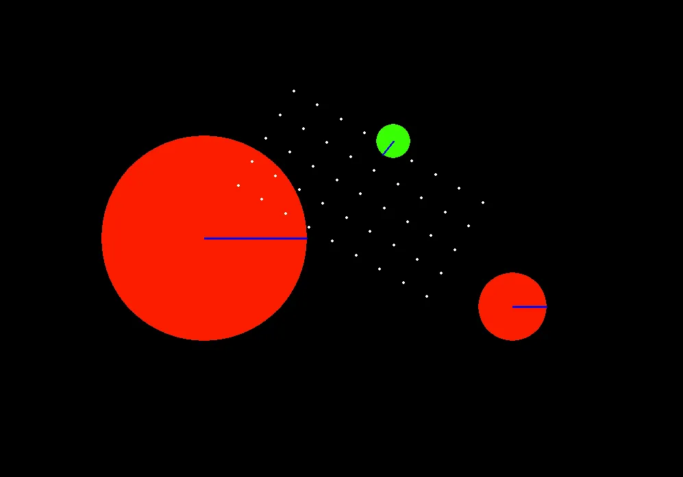
So I use a matrix of sensors that fan out the front of the car instead of an entire screen-worth of pixel data. These sensors read the pixel color at their location and convert that into a 0, 1 or 2 depending on if it’s come across an obstacle, a wall, or the open road. Now I realize I can’t get this reading from my apartment, either, but I figure it’s a step closer to the real thing.

Let’s get into it!

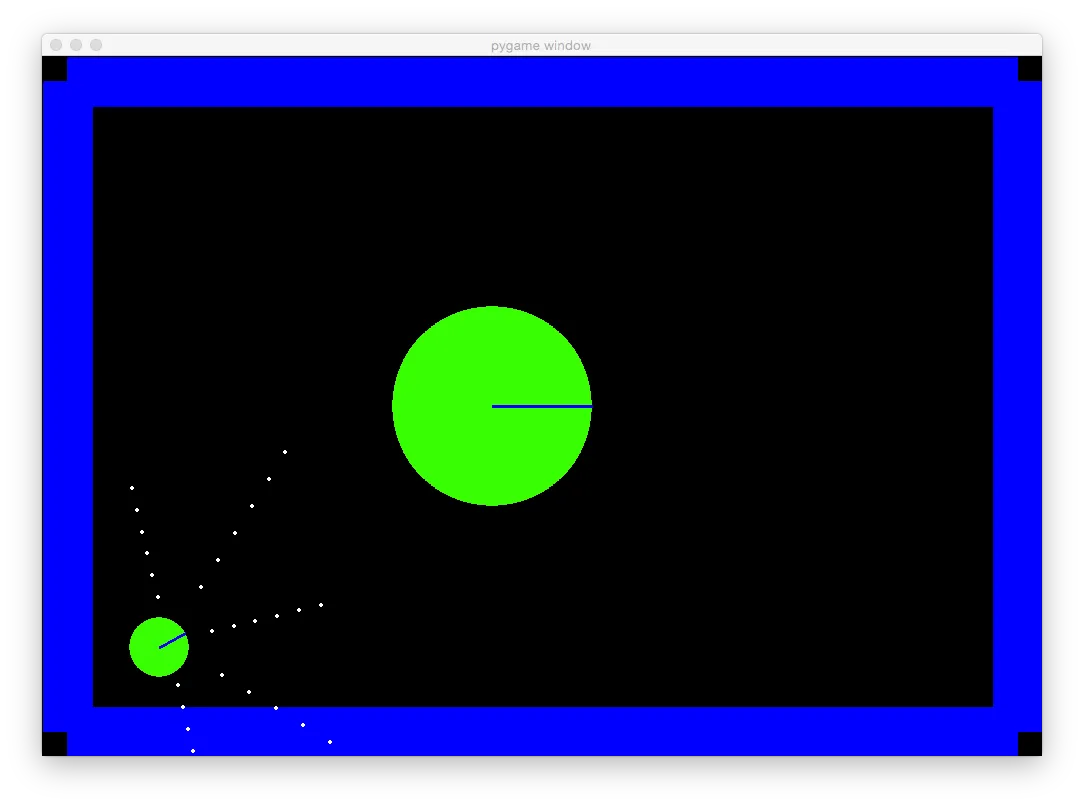
Screenshot of the first generation Robocar with its minimal fanned out sensors and single obstacle.

Libraries used

I used Python3 and Keras (with Theano backend) for the machine learning; Pygame and Pymunk for the game itself.

The code!

The code for this project is available on GitHub.

nn.py — This is where the Keras neural net lives.

carmunk.py — This is the game itself. The code is terrible and for that I apologize.

learning.py — Here lives the heart of the Q-learning process.

playing.py — Simply takes a trained model and drives!

Game controls, state and reward

The car automatically moves itself forward, faster and faster as the game progresses. If it runs into a wall or an obstacle, the game ends.

There are three available actions at each frame: turn left, turn right, do nothing.

At every frame, the game returns both a state and a reward.

The state is a 1d array of sensor values, which can be 0, 1 or 2, as stated above.

The reward is -500 if the car runs into something and 30 minus the sum of the sensor values if it doesn’t. The concept here is that the lower the sum of the sensors, the further away it is from running into something, and so we reward that. The -500 is a big punishment. How I came to choose -500, I don’t remember, but I believe it was in one of the code examples I reference in the credits above. I played around with different values and this one seemed to work best.

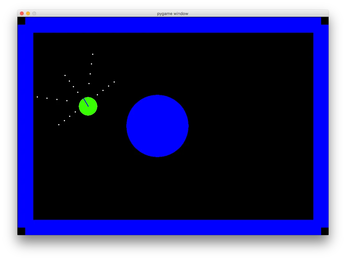
An earlier version of the game.

The learning algorithm

Outlace.com has done such a great job at explaining how Q-learning works that I won’t repeat it here. (I swear I’m not affiliated with that site or the author, I’m just ecstatic at how much the tutorials helped!) Instead, let me try to explain my implementation, step by step:

1. Start a new game and move the car forward one frame without turning.
2. Get a reading of the sensors.
3. Based on those readings, predict Q values. These predictions show Robocar’s confidence that it should take each of the three actions listed above. The first time through, these will be worthless, but we have to start somewhere.
4. Generate a random number. If it’s less than our epsilon (see below), choose a random action. If it’s higher than our epsilon, choose the most confident action returned from our prediction.
5. Execute the action (left, right, nothing) and get another sensor reading and our reward.
6. We store these things—the original reading, the action we took, the reward we got and the new reading—in an array that we call a buffer.
7. Grab a random sample of “reading, action, reward, new reading” from our buffer and learn by building an X, y training set that we “fit” our model to.
8. This is the most complicated part of the whole thing, and what I have the most trouble getting my head around. But let me try…
9. We set the y value for the iteration to a prediction based on the original reading.
10. We make a new prediction based on our new reading (post-action state).
11. We take a look at the reward we were given by taking the action. If it’s -500, we’ve run into something, and so we set the y for this iteration and this action to -500. If we didn’t run into anything, we multiply our max predicted Q value by a gamma (to discount it) and set the iteration’s y value for the action we took.
12. Go back to step 2 until we run into something.
13. When we run into something, decrease our epsilon and go back to step 1.

Here’s the code for steps 8 through 11:

def process_minibatch(minibatch):
    X_train = []
    y_train = []

    # Loop through our batch and create arrays for X and y
    # so that we can fit our model at every step.
    for memory in minibatch:
        # Get stored values.
        old_state_m, action_m, reward_m, new_state_m = memory

        # Get prediction on old state.
        old_qval = model.predict(old_state_m, batch_size=1)

        # Get prediction on new state.
        newQ = model.predict(new_state_m, batch_size=1)

        # Get our best move. I think?
        maxQ = np.max(newQ)
        y = np.zeros((1, 3))
        y[:] = old_qval[:]

        # Check for terminal state.
        if reward_m != -500: # non-terminal state
            update = (reward_m + (GAMMA * maxQ))
        else: # terminal state
            update = reward_m

        # Update the value for the action we took.
        y[0][action_m] = update
        X_train.append(old_state_m.reshape(NUM_SENSORS,))
        y_train.append(y.reshape(3,))

    X_train = np.array(X_train)
    y_train = np.array(y_train)

    return X_train, y_train

The whole “epsilon” thing

The epsilon helps us decide whether to explore a new action or take what we believe to be the best action available at any time. We start by always choosing a random action, because Robocar hasn’t learned anything. But over time, during training, the epsilon is decreased, and so we “randomly” choose the “best” action more often. The epsilon goes down to 0.1, so even at the end of the training cycle, it’s still choosing a random action 10% of the time.

The reason I mention it separately is that I ran into a funny issue. I spent hours of computation time trying out all sorts of different values and settings for just about everything in this project that has a mutable value or a setting. I couldn’t figure out why after all this training and learning, Robocar could still only achieve at most 22,000 frames of actions before running into a wall, and generally did much worse than that. (Note: This is for generation 1, which did not speed up over time.) I thought, “This thing is for sure going to run over my cats if it can’t even live for longer than 5 minutes going around circles.”

Then, I let the epsilon go below 0.1, all the way to 0. And when it did, the car never died. It just went round and round until I got bored and terminated it myself. Turns out, it had learned way more than I had realized.

So lesson learned: 10% of randomness can be a significant factor and may cause you to waste hours refining your settings when it would’ve done just fine all along.

The neural network

We use a relatively simple fully connected neural network as our model. We have three dense layers: input, a single hidden layer and output. We add a rectified linear units after the input and hidden layer to speed training, and also add a 0.2 dropout to prevent over-fitting. Given this isn’t a very complex problem, a lot of this (and the size of the hidden layer) is over-kill, but it’s fun to explore how different activations, dropout and hidden layer size impacts accuracy and training time. If you’ve downloaded the code, I encourage you to experiment with these parameters to see how they do for you.

The results

In the 1st gen with a single obstacle and no speed increase, Robocar drove flawlessly after very little learning. I’m talking infinite life after 10 minutes of training!

Here are some graphs that show the moving average of the distance it traveled (# of frames, averaged over 10 runs), from epoch 750–1000, with the epsilon decreasing slowly from 1 to 0.1. You can see that as it neared the finish, it often went through huge ups and downs. Honestly, I don’t entirely understand why. It seems that at some point, the network trains itself to go right, hard, and just runs itself into the wall over and over. Eventually it breaks out of that and then it performs really well for a couple games, before going back into wall banger mode. If anyone can explain why, I’d appreciate it.

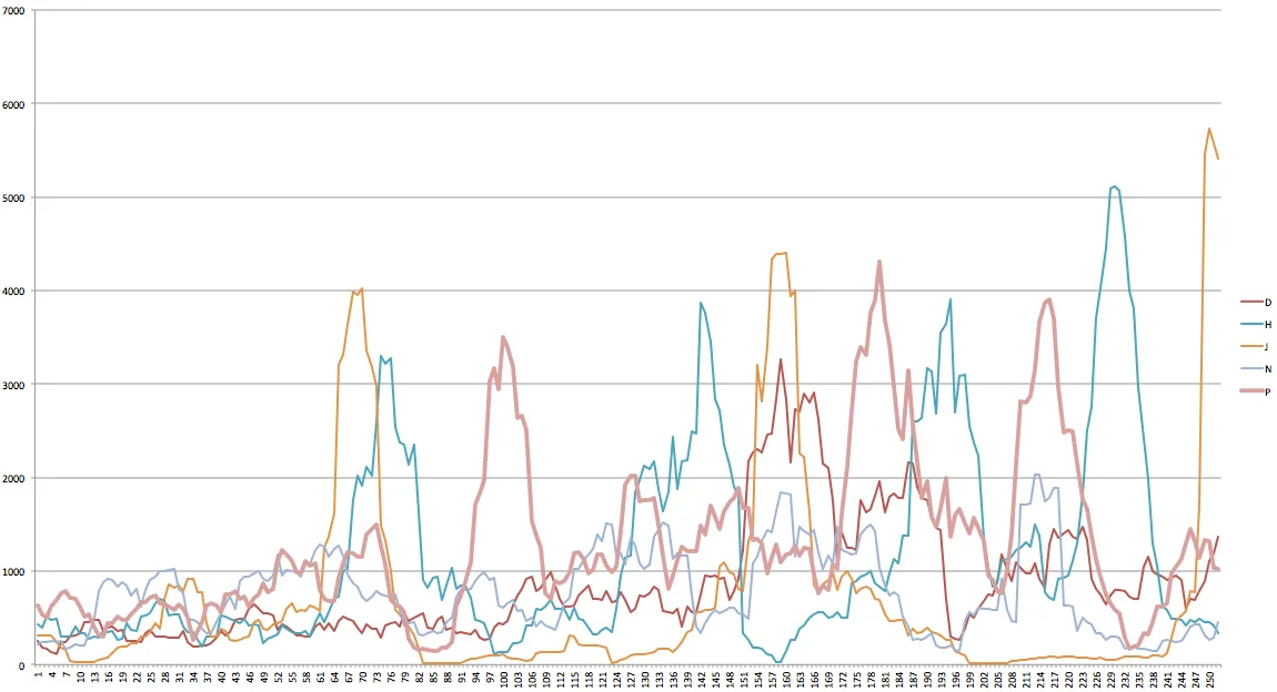
First gen moving average of distance for different settings. P, in pink, averaged the best results. It has a gamma of 0.9 and uses dropout of 0.2 on the NN. J, the strangest graph here, put up some huge numbers followed by periods of utter failure. Its gamma was at 0.999. N, the worst performer on this graph, had an extra hidden layer in the NN. This proves how little I know about neural nets…

I trained the 2nd gen version—consisting of somewhat randomly-generated obstacles, randomly generated starting corner and the new sensor matrix—using the best settings from the 1st gen, which is shown in series P in the graph above. All 1,000 gameplays, using a moving average of 10 games, results in the following learning pattern:

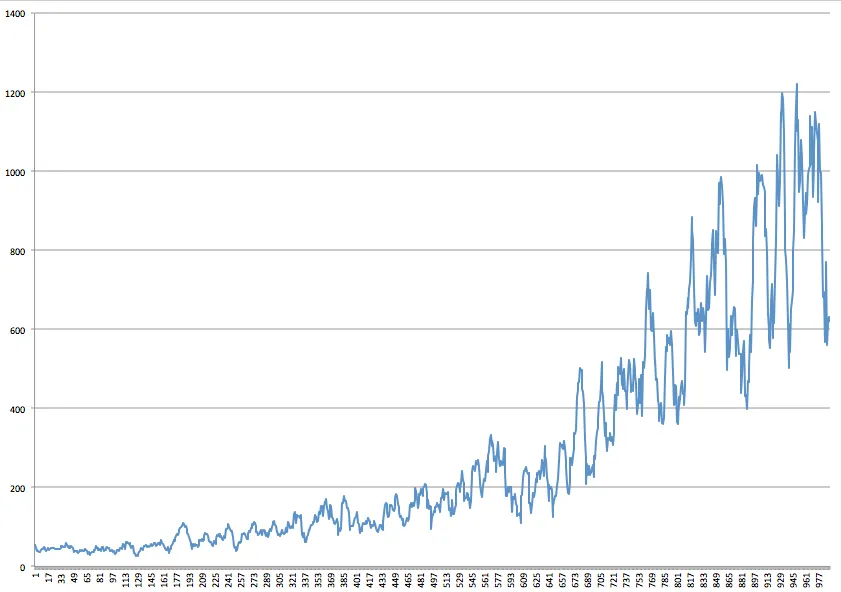
The Y-axis shows the average distance traveled over the previous 10 attempts. The scale is much smaller than the gen 1 graphs above, which is to be expected since this version is significantly more complex for Robocar. I’m glad to see that it does appear to be learning quite well. Let’s see how it looks when we play it!

And using the neural net weights from the top-performing game, we get this:

I think it does pretty well! What do you think?

Update, Feb 24, 2016: Be sure to take a look at part 2 where I analyze the loss, do some parameter tuning and display some pretty graphs: Reinforcement learning in Python to teach a virtual car to avoid obstacles — part 2

Update, March 7, 2016: Part 3 is now available. Here, we convert our sim into something that gets us closer to a real-world model.

In case you missed the link above, all the code is available on GitHub here: Reinforcement Learning Car with Python