Reinforcement learning in Python to teach a virtual car to avoid obstacles — part 2

Something that bothered me after publishing part 1 of my exploration of reinforcement learning was how I measured success. I logged the distance the car traveled in each “game” (epoch), plotted it, looked at the graph and then said, “Yep, looks like it’s learning.”

Update, March 7, 2016: Part 3 is now available. We take the next step in turning the simulation into a real-world ready model.

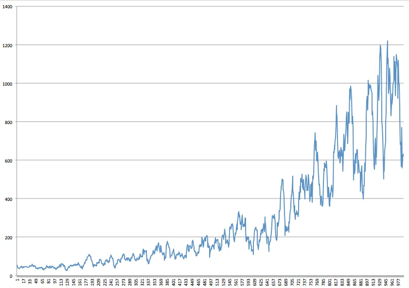
Example of a distance graph from part 1.

I was able to verify that it was actually learning quite well and even more quickly than I had realized. However, there was too much randomness in the result. Depending on the randomly selected assortment of obstacles and the starting position of the car plus the fact that at its least random it chose a random action 10% of the time (epsilon-greedy!), could I really tell how reliable the metrics were?

Then I realized: The neural net measures the loss at each training step, and I’m discarding this metric like it’s dirt.

Oh, the ignorance!

If you look at the more recent version of the code, you’ll see that I now record the loss at each step. I’ve also created a way to plot the loss (and distance) to make it easier to visualize. Another big change I made was to alter the epoch style. Instead of limiting training to a specific number of games, it now performs a specific number of frames, no matter how well it does per game. This is because previously if the learner wasn’t doing so hot, it would train for far less time than the faster but potentially less effective learners.

Using loss for hyper parameter tuning

With the loss reading now at our side, the next step was to do some hyper parameter tuning. Specifically, I wanted to explore the following parameters:

• Number of hidden neurons per layer: 20x20, 164x150, 256x256, 512x512, 1000x1000
• Batch size: 32, 40, 100, 400
• Buffer (experience replay): 10,000, 50,000, 500,000
• Gamma: 0.9, 0.95

After running 250,000 frames of training for each of the 60 combinations of the first three params (plus a random sample to test the gamma), some interesting patterns emerged.

Interesting patterns

1. The smaller the buffer size, the lower the loss but greater the variance. At a large 500,000 replay buffer, there’s a tiny amount of variance but very little learning. 10,000 just looks like a highly variant 50,000. So 50,000 might be a sweet spot.
2. The bigger the network the lower the loss. However, the bigger networks also had a lower max distance and average distance per game. It’s likely that this is because the network trains more slowly. This isn’t necessarily a bad thing. (Todo: Run a big network for a million frames and observe.)
3. The bigger the batch size the lower the loss and the lower the variance. Unfortunately, the bigger the batch size, the slower it is to train.
4. Gamma at 0.9 is better than 0.95 across the board.

What’s this all mean? A few scenarios

Scenario #1: The biggest, slowest, most complex networks look good but will require a lot more training. (1000 x 1000 hidden neurons, 400 batch size with 10,000 replay experience had the lowest loss.)

Scenario #2: 512 x 512 at 400 and 50,000 looks like a good tradeoff since it’s a little faster and appears to be learning quickly and smoothly.

Scenario #3: Interesting curveball: Hidden layers of 164 x 150 neurons with 400 batch size and 50,000 buffer may be the best compromise of them all (see graphs below).

Graphs below

As a baseline: A 20 x 20 neural network with a batch size of 32 and a 50,000 buffer:

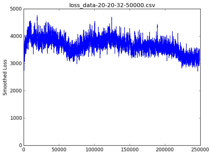
High loss, lots of variance, not a lot of learning going on.

Scenario #1: 1000 x 1000, 400 batch size, 10K buffer:

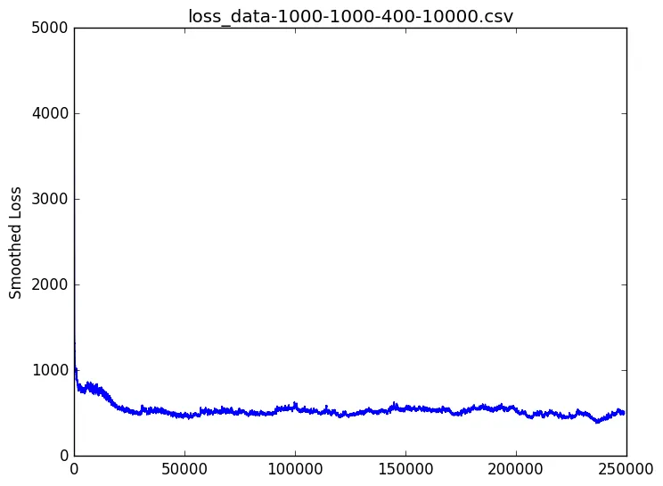
Very low loss, low variance, but also a flat learning rate.

Scenario #2: 512 x 512, 400 batch size, 50K buffer:

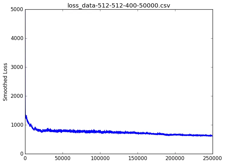
Low loss, low variance, continuous (slow) learning. Looks promising.

Scenario #3: 164 x 150, 400 batch size, 50K buffer:

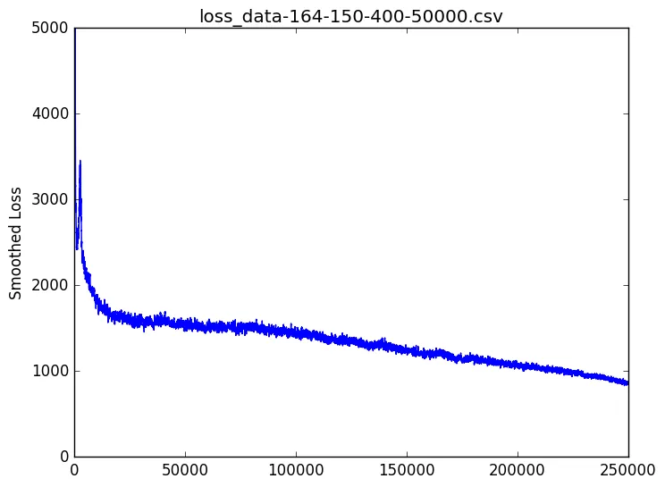
Look at that slope! This is perhaps most promising. It has a higher absolute loss than numbers 1 and 2 but a good learning rate that shows good potential and it’s much faster to learn than the larger networks.

And here’s the smoothed distance graph for scenarios #1 and #3:

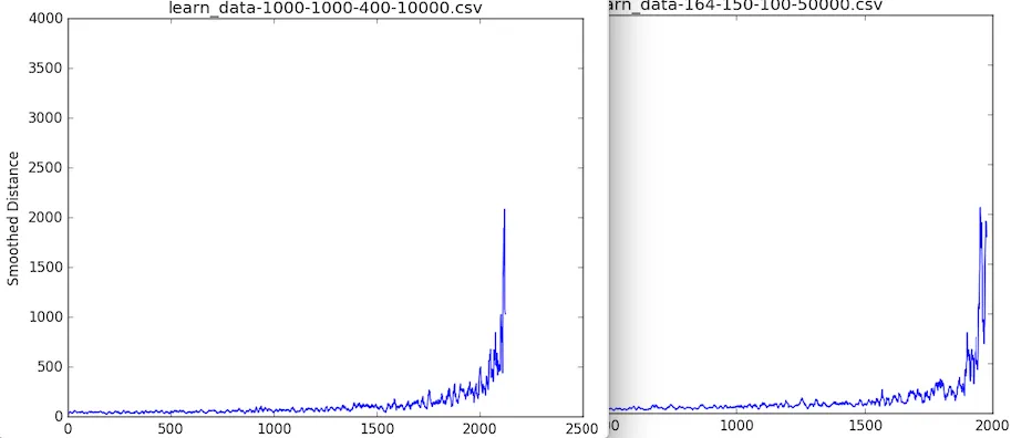
Both look promising.

What’s next?

If you recall from part 1, the end goal of all of this is to train a remote control car to drive itself around my apartment without running into my cats. So now that we have a decent understanding of our network, it’s time to make some changes to the simulation:

1. We can’t get “pixel readings” at a matrix of points in front of and beside the car. Instead, we’ll have to use ultrasonic sensors. So change the input to be the a reading of three distances from the car to any object it detects. With this, we also have to update our reward function.
2. In real life, we can’t reset the car to its starting point when it crashes, so we need a recovery algorithm.
3. We can’t set a collision flag to true when we bump into something, so we need to use the sensor readings to detect a crash in order to initiate the recovery algorithm.
4. Cats aren’t stationary: We’re going to need some dynamic obstacles.

Update, March 7, 2016: Part 3 is now available. We implement these four steps, turning the simulation into a real-world ready model.

Aside: Making Pygame really, really fast

One of the challenges of this learning versus learning ML algorithms on data is that we have an actual game that we have to control. And let’s face it, redrawing a screen is SLOW. But I figured out a great trick: you don’t actually have to redraw the screen at all! Simply commenting out the flip() call makes the game itself run at north of 300 frames per second. (I’ve seen it as high as 600 fps.) Of course once it starts training the net it slows down, but not redrawing the screen essentially takes the game out of the time equation altogether without impacting its ability to learn.

If you’re looking for the code, take a look here: Using reinforcement learning to teach a car to avoid obstacles.